Butterfly drawing mechanism

Design of Drawing Mechanisms

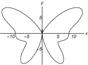
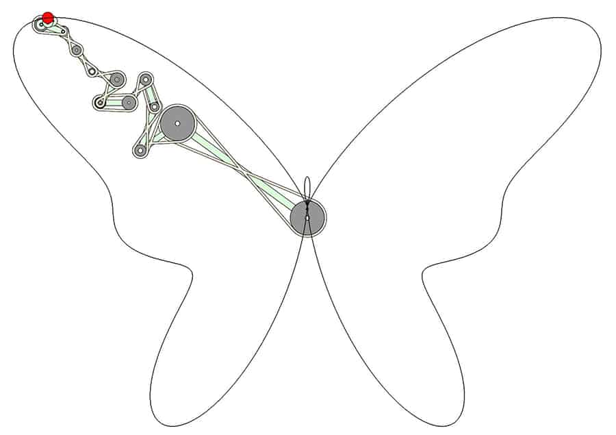
Mechanical systems that draw trigonometric curves provide a versatile way to draw complex curves. Yang Liu designed this serial chain consisting of 14 links coupled by a belt drive to draw the Butterfly curve.


The Butterfly curve is an example of a trigonometric plane curve, and our study of Kempe’s design of linkages to draw algebraic curves has lead us to a way to design serial chains that draw these curves.

Here is how it is done.

Butterfly curve

Butterfly curve

Trigonometric curves. A trigonometric plane curve is a parametrized curve with coordinate functions, P = (x, y), that are finite Fourier series,

Trigonmetric equation

Trigonmetric equation

where ak , bk , ck and dk are real coefficients and theta ranges from 0 to $latex 2\pi$.

A large number of well-known curves have this form, such as Limacon of Pascal, the Cardioid, Trifolium, Hypocycloid and Lissajous figures.

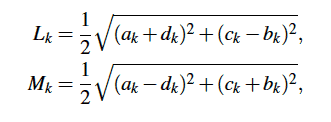
A coupled serial chain. Without going into too much detail, it is possible to use the coefficients ak , bk, ck and dk to define the link dimensions,

Link dimensions

Link dimensions

and the initial angles,

Initial angles

Initial angles

These parameters allow us to redefine the trigonometric equations of the curve as the coordinate equations of the links of a serial chain,

Serial chain equations

Serial chain equations

This equation identifies the curve as the end of a serial chain consisting of a sequence of links L1, M1, L2, M2 and so on, such that the Lk links rotate counter clockwise and the Mk links rotate clockwise both at the rate $latex k\theta$.

The initial angles define the configuration of the serial chain when  $latex \theta=0$.

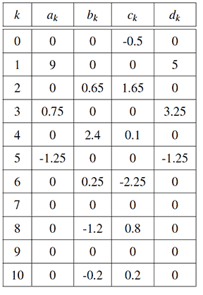
The Butterfly drawing mechanism. The trigonometric curve of the Butterfly linkage is defined by the coefficients in the following table,

Table of Butterfly coefficients

Table of Butterfly coefficients

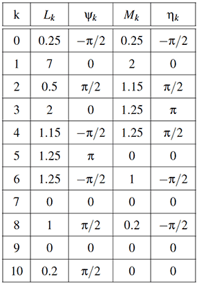
These coefficients are used to calculate the dimensions and initial configuration of the serial chain listed in the following table,

Table of Butterfly link dimensions

Table of Butterfly link dimensions

The result is a serial chain consisting of 14 links that are coordinated to move together as the base rotates. The end-point of the chain draws the Butterfly curve.

Butterfly drawing mechanism

Butterfly drawing mechanism

Mechanisms and Robotics Conference

2016 Mechanisms and Robotics Conference

Mechanisms and Robotics Conference

Symposia organized for the 2016 Mechanisms and Robotics Conference

The 2016 Mechanisms and Robotics conference is part of International Design Engineering Technical Conferences organized by ASME International in Charlotte, North Caroline, August 22-24.

Plenary speaker Bernard Roth is the Academic Director of Stanford University’s d.school and the author of the Achievement Habit.

For some reason, ASME has broken these links to the 2016 IDETC conference, but you can find out more about each of the symposia at the conference overview link: 2016 ASME Mechanism and Robotics Conference Overview.  Then select the Expand all Symposia Link to see the sessions and a list of papers.


MotionGen Horse

Motion Gen Linkage Design App

MotionGen is a planar four-bar linkage simulation and synthesis app that helps users synthesize planar four-bar linkages by assembling two of the planar RR-, RP- and PR-dyad types, (R refers to a revolute or hinged joint and P refers to a prismatic or sliding joint).

The input task is a planar motion given as a set of discrete positions and orientations and the app computes type and dimensions of synthesized planar four-bar linkages, where their coupler interpolates through the given poses either exactly or approximately while minimizing an algebraic fitting error.  The algorithm implemented in the app extracts the geometric constraints (circular, fixed-line or line-tangent-to-a-circle) implicit in a given motion and matches them with corresponding mechanical dyad types enumerated earlier.  In the process, the dimensions of the dyads are also computed. By picking two dyads at a time, a planar four-bar linkage is formed. Due to the degree of polynomial system created in the solution, up to a total of six four-bar linkages can be computed for a given motion.


MotionGen display

MotionGen display

MotionGen also lets users simulate planar four-bar linkages by assembling the constraints of planar dyads on a blank- or image-overlaid screen. This constraint-based simulation approach mirrors the synthesis approach and allows users to input simple geometric features (circles and lines) for assembly and animation. As an example of the Simulation capabilities of the app, Figure shows a walking robot driven by two sets of planar four-bar linkages where the foot approximately traces a trajectory of walking motion. The users can input two dyads on top of an imported image of a robot or machine to verify the motion and make interactive changes to the trajectories.

Anurag Purwar describes MotionGen and its applications in this video:

MotionGen is available as a free download at both Google Play- and Apple’s iTunes-Stores.


Elliptic curve drawing

Mechanical computation and algebraic curves

A mechanical computer that draws an algebraic curve is a useful device, and  Mathematicians Michael Kapovich and John Millson have shown that a design always exists.

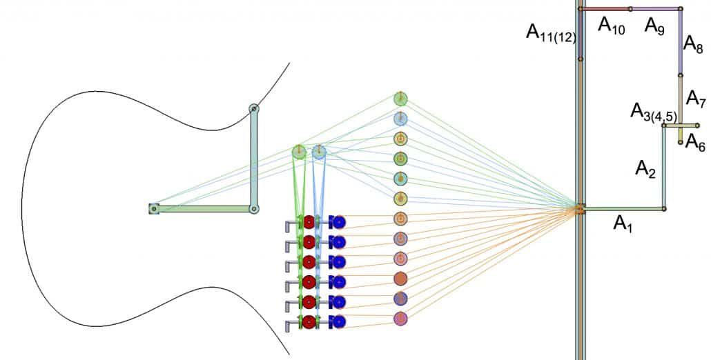
This is Yang Liu’s design of a mechanical system that draws an elliptic cubic curve.

Here is how it is done.

Algebraic curve. An algebraic curve is the set of points P=(x, y) with coordinates that satisfy an algebraic equation,

Algebraic curve

 Algebraic curve

where ui and vi are integer exponents, and ci are real coefficients.

Forward kinematics. In order to draw this curve, we use an RR serial chain shown in Figure 1.  All that is needed is to coordinate the angles of this chain so its end-point P traces the curve.

RR serial chain

 Figure 1. The joints of an RR serial chain are coordinated to guide the point P along a specified curve.

The relationship between the joint angles and the coordinates P=(x, y) is given by the forward kinematics equations of this RR chain,

RR forward kinematics

 RR forward kinematics

Kempe’s formula. In his 1876 paper, “On a general method of describing plane curvesof nth degree by linkwork,” A. B. Kempe substituted this into the equation of the curve and simplified the result to obtain,

Kempe formula

 Kempe formula

Kempe interpreted this formula to be the x-coordinate of an N link serial chain, where each link has the length Aj and is positioned at the angle,

Kempe link angles

 Kempe link angles

The end-point of Kempe’s serial chain maintains the value x=C, which means it only moves along the y-direction.

Mechanical computation. Now connect cable drives to the two joints of the RR chain so they can be used as inputs to N mechanical computers that calculate the Psij angular values.  The output of the mechanical computers are connected by cable drives to the joints of Kempe’s serial chain.

The operations needed in the mechanical computers are simply multiplication and addition.  Multiplication of an angle by a given factor is achieved by using a cable drive with the ratio of the pulley sizes set to the specified factor.  The sum of two angular values is achieved using a bevel gear differential.

The result is a mechanical system that constrains the angles of an RR chain so it draws the specified algebraic curve within the workspace of RR serial chain.

Elliptic cubic curve. As an example, consider the elliptic cubic curve,

Elliptic cubic curve

 Elliptic cubic curve

Let the RR chain have link lengths L1=L2=1, and obtain Kempe’s formula for this curve,

Elliptic cubic formula

 Elliptic cubic formula

This equation has 12 terms, so Kempe’s serial chain has 12 links. The 12 mechanical computers connecting the angles of Kempes serial chain to the driving joints for the RR chain, include six additions and eight multiplications, Figure 2.

Elliptic curve drawing

 Figure 2. The Kempe’s serial chain and the mechanical computations that constrain the RR serial chain to draw an elliptic cubic curve.

Rather than use differentials and cable drives, Kempe used linkages to perform the mechanical computations and couple the results. The outcome is a lot of links as can be seen in this animation provided by Alex Kobel.

Trifolium Contra-parallelograms

Trifolium using contra-parallelograms

Trifolium Contra-parallelograms

Trifolium Contra-parallelograms

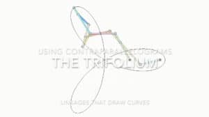
Yang Liu shows that a simple linkage can draw the trifolium curve.

For comparison here is the Kempe linkage that draws a trifolium curve obtained by Alexander Kobel.

Linkage Patents

Want a patent? Try a Six-bar linkage

Patents including six-bar linkages are rare. Thousands of U.S. Patents have been awarded over the past forty years that involve four-bar linkages, but less than a hundred involve six-bar linkages, Figure 1.

Linkage Patents

Figure 1.  Since 1976, 3619 patents have been awarded that involve four-bar linkages and only 84 that involve six-bar linkages.

Add two bars to a four-bar to get a six-bar. A four-bar linkage, familiar to all mechanical designers, has an input lever connected by a rod to an output lever, Figure 2 (top). Add two more bars and you have a six-bar linkage. Unfortunately, the standard way to add those bars yields sequence of two four-bar linkages, Figure 2 (bottom), which is not really new. There are other ways to add these two bars but they are beyond the state-of-the-art.

Six-bar Watt 2

Figure 2. Add two bars to a four-bar linkage (top) to obtain a sequence of two four-bar linkages (bottom). This is the best designers can currently do for a six-bar linkage.

Other ways to add two bars. The two additional bars can be added to a four-bar linkage by attaching one end to the connecting rod and the other end to the output link. The result is a stack of two four-bar linkages, known as the Watt I six-bar linkage, Figure 3(a).

Another way is to connect one end of the two bars to the input lever and the other to output lever. This can be done in two ways, either on top of or beneath the four-bar linkage. When added on top, the result is a five-bar loop stacked on the four-bar linkage, known as the Stephenson I six-bar, Figure 3(b). When added beneath, the four-bar linkage is stacked on a five-bar loop, which is a Stephenson II sixbar, Figure 3 (c).

A systematic procedure for design of these alternative six-bar linkages is simply not available to mechanical designers.
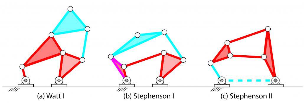
Six-bar Chains

Figure 3. Three ways to add two bars to a four-bar linkage to obtain a six-bar linkage, each of which is beyond the state-of-the-art.

Solving the loop equations for four-bar and six-bar linkages. There is a simple, though mathematical, reason why four-bar linkages are easy to design and six-bar linkages that are more than a sequence of two four-bar linkages are very hard to design.

Almost sixty years ago in 1954, Ferdinand Freudenstein showed that if we define the movement required of a four-bar linkage, then its dimensions can be computed from its loop equations, which in modern form are give by,

Four-bar Loop Equations

Four-bar Loop Equations

He also showed that the solution of these equations is equivalent to finding the roots of a fourth degree polynomial, which is easy to do.

Soon afterward researchers obtained two sets of loop equations for six-bar linkages and showed that for a required movement, the solution of its loop equations,

Six-bar Loop Equations

Six-bar Loop Equations

is equivalent to finding the roots of a polynomial system of degree, d=264×10^6. A complete solution was only recently achieved after 300 hours of computation on a high performance computer cluster.

This stunning increase in complexity gets worse for eight-bar linkages obtained by adding two bars to a six-bar linkage, which yields three sets of loop equations. In this case calculating the dimensions of the linkage involves the solution of a polynomial system estimated to be of degree, d=10^15, which is massively beyond capabilities of even theoretical polynomial solvers.

A four-bar with additional design parameters. Once we understand the structure of the design equations for four-bar, six-bar and even eight-bar linkages, it is possible to take a different approach to the problem of calculating a design from a movement requirement.

A four-bar linkage has eight design variables, which are the four pairs of coordinates that define its hinged joints. Similarly, a six-bar linkage has seven hinged joints or 14 design parameters, and an eight-bar linkage has 10 joints or 20 design parameters. It is possible to consider a six-bar and even an eight-bar linkage as a four-bar linkage with extra design variables. The question then becomes how to use these extra design variables to improve the performance of the linkage system.

Six-bar linkages provide simple and effective movement. But is there ever a situation where the complexity of a six-bar linkage is preferred over a four-bar linkage that provides the same movement? Of course there is, but let’s let design engineers describe their experience.

Søren Matthesen, design engineer for Vendlet Aps, which makes automated equipment for beds, studied the use of gears, guide rails and four-bar linkages and wound up using a six-bar linkage for his application. He states,

“What really mattered to me was the fact that the six-bar linkage enabled me to solve my design task unlike the four-bar linkage. This is a huge advantage in functionality. Compared to my initial solutions, the six-bar linkage system ends up being more simple and stable to produce, use and maintain.”

Mike Sutherland, design engineer, Zennen Engineering, designed a six-bar linkage to fold the rear wheel of a new full-scale folding bicycle, Figure 4. He states,

“The six-bar rearstay folding linkage provided very tight package; that besides being convenient for transportation, also has something of a ‘Transformer’ attraction about it…”

Zennen Folding Bike

Figure 4. The Zennen folding bicycle concept uses a six-bar linkage to fold the full-sized rear wheel against the folded front forks, downtube and seat tube.

The simple answer is that a six-bar linkage designed to achieve the same movement as a four-bar linkage will have free design parameters that allow optimization of other features important to the designer, and this definitely justifies the increase in complexity. And it may be an invention ready for a U. S. Patent.

2015 Energy Invitational

2015 UCI Energy Invitational Video

This video shows highlights of the 2015 Energy Invitational on UCI’s Campus:

The 2016 UCI Energy Invitational will be May 21, 2016 on UCI’s Campus. The course will be along East Peltason Drive between Los Trancos and Bison.

2016 Energy Invitational

2016 Energy Invitational

Fourier Curve Tracing

Fourier Curve Tracing

Fourier Curve Tracing

Fourier Curve Tracing


This animation by Yang Liu is inspired by the mechanical Fourier synthesizer described by Dayton Miller, see A 32-element harmonic synthesizer.

This mechanical system combines the terms of a Fourier approximation of the batman curve found on Wolfram.com. The video below shows this device draws the batman curve.

SIAM News

SIAM News: Biologically inspired linkage design

SIAM News

SIAM News

This article by Jon Hauenstein with me for SIAM News (Society for Industrial and Applied Mathematics) describes research by Mark Plecnik in the computer-aided design of linkages to provide mechanical movement of a bird’s wing. Here is Mark’s video of the his wing flapping mechanism.

Epsilon is ready

Epsilon is ready for the LA Auto Show

Epsilon is ready

Epsilon is ready

See Epsilon at the 2015 LA Auto Show. This former FSAE racecar is now UCI’s research vehicle for an innovative torque-vectoring electric drive system. The body is by a team at the Art Institute of Orange County.