August 2016

2016 Mechanisms and Robotics Conference

August 13, 2016/by Prof. McCarthy

Symposia organized for the 2016 Mechanisms and Robotics Conference

The 2016 Mechanisms and Robotics conference is part of International Design Engineering Technical Conferences organized by ASME International in Charlotte, North Caroline, August 22-24.

Plenary speaker Bernard Roth is the Academic Director of Stanford University’s d.school and the author of the Achievement Habit.

For some reason, ASME has broken these links to the 2016 IDETC conference, but you can find out more about each of the symposia at the conference overview link: 2016 ASME Mechanism and Robotics Conference Overview. Then select the Expand all Symposia Link to see the sessions and a list of papers.

Motion Gen Linkage Design App

August 8, 2016/by Prof. McCarthy

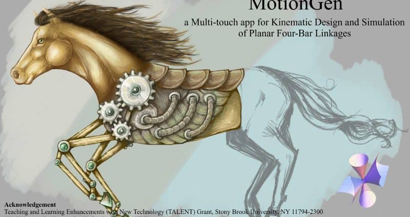
MotionGen is a planar four-bar linkage simulation and synthesis app that helps users synthesize planar four-bar linkages by assembling two of the planar RR-, RP- and PR-dyad types, (R refers to a revolute or hinged joint and P refers to a prismatic or sliding joint).

The input task is a planar motion given as a set of discrete positions and orientations and the app computes type and dimensions of synthesized planar four-bar linkages, where their coupler interpolates through the given poses either exactly or approximately while minimizing an algebraic fitting error. The algorithm implemented in the app extracts the geometric constraints (circular, fixed-line or line-tangent-to-a-circle) implicit in a given motion and matches them with corresponding mechanical dyad types enumerated earlier. In the process, the dimensions of the dyads are also computed. By picking two dyads at a time, a planar four-bar linkage is formed. Due to the degree of polynomial system created in the solution, up to a total of six four-bar linkages can be computed for a given motion.

MotionGen display

MotionGen also lets users simulate planar four-bar linkages by assembling the constraints of planar dyads on a blank- or image-overlaid screen. This constraint-based simulation approach mirrors the synthesis approach and allows users to input simple geometric features (circles and lines) for assembly and animation. As an example of the Simulation capabilities of the app, Figure shows a walking robot driven by two sets of planar four-bar linkages where the foot approximately traces a trajectory of walking motion. The users can input two dyads on top of an imported image of a robot or machine to verify the motion and make interactive changes to the trajectories.

Anurag Purwar describes MotionGen and its applications in this video:

MotionGen is available as a free download at both Google Play- and Apple’s iTunes-Stores.

Mechanical computation and algebraic curves

August 3, 2016/by Prof. McCarthy

A mechanical computer that draws an algebraic curve is a useful device, and Mathematicians Michael Kapovich and John Millson have shown that a design always exists.

This is Yang Liu’s design of a mechanical system that draws an elliptic cubic curve.

Here is how it is done.

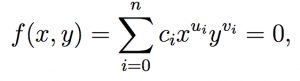
Algebraic curve. An algebraic curve is the set of points P=(x, y) with coordinates that satisfy an algebraic equation,

Algebraic curve

where u_i and v_i are integer exponents, and c_i are real coefficients.

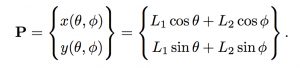
Forward kinematics. In order to draw this curve, we use an RR serial chain shown in Figure 1. All that is needed is to coordinate the angles of this chain so its end-point P traces the curve.

Figure 1. The joints of an RR serial chain are coordinated to guide the point P along a specified curve.

The relationship between the joint angles and the coordinates P=(x, y) is given by the forward kinematics equations of this RR chain,

RR forward kinematics

Kempe’s formula. In his 1876 paper, “On a general method of describing plane curvesof nth degree by linkwork,” A. B. Kempe substituted this into the equation of the curve and simplified the result to obtain,

Kempe formula

Kempe interpreted this formula to be the x-coordinate of an N link serial chain, where each link has the length A_j and is positioned at the angle,

Kempe link angles

The end-point of Kempe’s serial chain maintains the value x=C, which means it only moves along the y-direction.

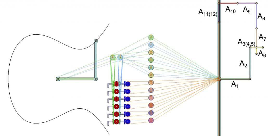
Mechanical computation. Now connect cable drives to the two joints of the RR chain so they can be used as inputs to N mechanical computers that calculate the Psi_j angular values. The output of the mechanical computers are connected by cable drives to the joints of Kempe’s serial chain.

The operations needed in the mechanical computers are simply multiplication and addition. Multiplication of an angle by a given factor is achieved by using a cable drive with the ratio of the pulley sizes set to the specified factor. The sum of two angular values is achieved using a bevel gear differential.

The result is a mechanical system that constrains the angles of an RR chain so it draws the specified algebraic curve within the workspace of RR serial chain.

Elliptic cubic curve. As an example, consider the elliptic cubic curve,

Elliptic cubic curve

Let the RR chain have link lengths L₁=L₂=1, and obtain Kempe’s formula for this curve,

Elliptic cubic formula

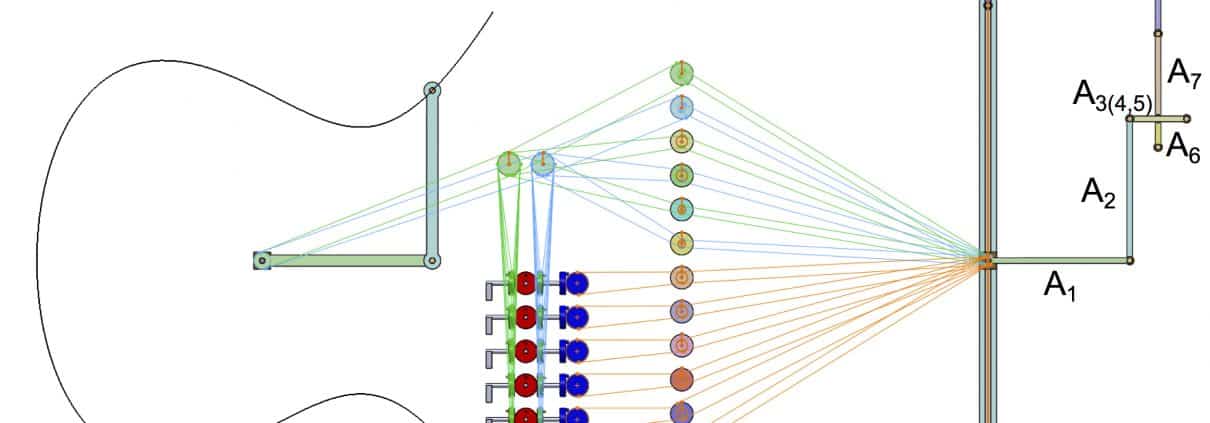
This equation has 12 terms, so Kempe’s serial chain has 12 links. The 12 mechanical computers connecting the angles of Kempes serial chain to the driving joints for the RR chain, include six additions and eight multiplications, Figure 2.

Figure 2. The Kempe’s serial chain and the mechanical computations that constrain the RR serial chain to draw an elliptic cubic curve.

Rather than use differentials and cable drives, Kempe used linkages to perform the mechanical computations and couple the results. The outcome is a lot of links as can be seen in this animation provided by Alex Kobel.